This week, we hit a major milestone: our solver can now complete very easy Sudoku puzzles, thanks to the simplest rule of all — the single candidate rule. By writing code that parses the grid repeatedly and looks for opportunities to apply this rule, we’re able to solve some of the simplest Sudoku puzzles and our app is finally achieving its goal for those puzzles.
The current code at the time of writing can be found on GitHub where you can also see the pull request for the changes in this post.
If you like this post and you’d like to know more about how to plan and write Python software, check out the Python tag. You can also find other posts in the Sudoku Series.
What is the Single Candidate Rule?
While the single candidate rule is often used in tandem with more advanced techniques, some puzzles (especially very easy ones) can be solved using this rule alone.
Under the single candidate rule, the cells of the grid that are currently unsolved must take note of all the possible candidates for the cell. This means they consider all the digits from 1 through 9 as candidates and look at their neighbouring cells for solved values, removing those from the candidates. After this step, if a cell only has one candidate left, that means this cell must contain that value. You can add the value to the cell to make it solved, and must also remove that value from the candidates of all its neighbouring cells.
Identifying Candidates
Immediately after creating the grid from the inputs, we can work out the candidates for every unsolved cell. Since we already built the methods that pull out the set of neighbours for a given cell, that makes this process surprisingly simple.
Here’s the method that initializes candidates for each unsolved cell, based on its neighbours:
for cell in self:
    if cell.value is not None:
        continue

    cell.candidates = set(range(1, 10))
    neighbours = self.get_neighbours(cell)
    n_values = {n.value for n in neighbours if n.value is not None}
    cell.candidates -= n_values
This iterates over the cells of the grid, skipping any that already have a value. For those without a value, the candidates list is initialised to a set of the values 1 through 9. The neighbours of the cell are discovered and their values, if they have any, are combined in a second set. This second set is subtracted from the initialised set of 1 through 9, to give the complete list of candidates for the cell.
Solving the Grid
Now that we have all the candidates set for the grid, we can hand the grid to a new Solver class.
The solve() method on this class will apply all the rules we have in an endless loop until we cannot apply any of our rules any more.
At this point, either the puzzle is solved, it’s unsolvable or we would need to implement more rules to be able to solve it.
The Solve Loop
The solve() method is implemented as shown here.
For now, we only have one rule to apply.
while True:
    applied = False

    # Apply rules
    applied |= solve_single_candidates(self.grid)

    # If no rules were applied, we cannot proceed further
    if not applied:
        break
The loop runs as many times as it needs to while rules continue to declare they have made changes to the grid.
We reset the applied variable to False every loop, before trying to update it by asking the single candidate rule to apply itself to the grid.
If the rule made any changes, it will return True and applied will become True.
The or-and-assign function |= ensures that the applied value can change from False to True when the value on the right gives a True value, but if the value on the right is False this doesn’t change applied to False.
In other words, once any rule in the loop changes the grid, applied changes to True and stays that way until the end of the loop.
As long as applied has changed to True by the end of the loop, we go back to the beginning, only breaking out of the loop when no more rules can be applied to the grid.
The Single Candidate Rule Code
The code for the single candidate rule is not very complicated.
applied = False

for cell in grid:
    if cell.value is not None:
        continue

    if len(cell.candidates) == 1:
        set_cell_value(grid, cell, cell.candidates.pop())
        applied = True

return applied
We once again have an applied variable which we initially set to False.
Looping over all the cells of the grid, we skip to the next cell if the one being considered already has a value.
For those without a value, if the number of candidates for the cell is exactly one, we set its solved value to the candidate and change our applied variable to True.
After all cells have been iterated over, we return the value of applied.
Setting a Cell Value
Lots of rules we will implement in the future are going to need to set values on cells as part of the solve. This isn’t as simple as setting the value and calling it a day, as we also need to update candidates for neighbouring cells. Since we don’t want to keep duplicating this code, it made sense to move the implementation out to a different file all the rules can use.
cell.value = value

incomplete_neighbours = (
    neighbour for neighbour in grid.get_neighbours(cell) if neighbour.value is None
)

for neighbour in incomplete_neighbours:
    neighbour.candidates = neighbour.candidates.difference({cell.value})
The method sets the value on the cell before finding all the unsolved neighbouring cells using a list comprehension with a filter. For each of those unsolved neighbours, the set difference ensures the new value is removed from their candidates list. This might enable those cells to be solved with the single candidate rule when they are next considered as part of the solving loop.
Checking Grid Validity and Solved State
The Solver class also implements two methods to check the grid’s validity and its solved state.
We can check whether a grid is solved or not simply by checking whether all the cells now hold a solved value.
return all(cell.value is not None for cell in self.grid)
Checking whether the grid is valid is actually only checking whether any cell’s solved value clashes with the solved value of a neighbour.
This should only be able to return False after loading the initial grid since our rules should never cause a conflict.
for cell in self.grid:
    if cell.value is not None and any(
        neighbour.value == cell.value
        for neighbour in self.grid.get_neighbours(cell)
    ):
        return False

return True
For each cell in the grid, we will return False if the value of the cell is not None (i.e. it is solved) and any of its neighbours have the same solved value.
If none of the cells meet this criteria, the grid is valid and we return True.
Note that this doesn’t check that the grid is solvable. That is only determinable after we try to apply all our rules to completion and relies on our rules being able to handle every possible solving scenario.
Seeing the Results
In order to see the state of the Sudoku grid while we work on rules, it felt sensible to allow rendering to graphic files.
Since the existing ASCII rendering of the grid felt like it should be a core function of the Grid class, this was moved to a new util script for grid rendering.
Alongside it, we implement a PIL.Image based rendering function to get images out as seen below.
Very Easy Grid
Loading the puzzle for Very Easy 2 and rendering gives us the following grid.

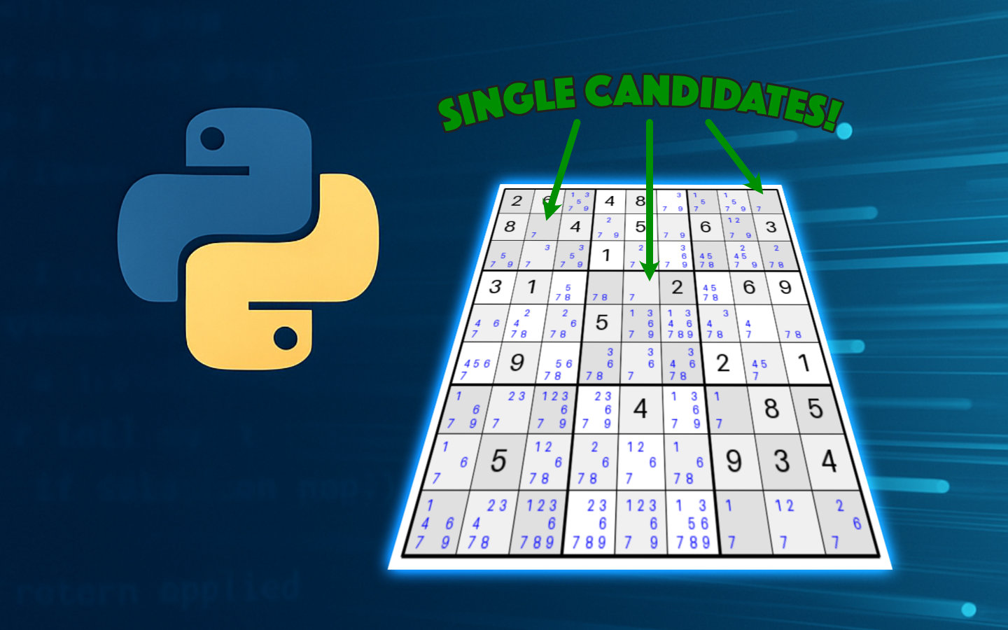
While it’s not clear that this puzzle has available single candidates, we can add the candidates to the grid and render it again.

Two of the starting cells have a single candidate 7 in them and these would be the first cells to be populated with a value. Immediately afterwards, some of their neighbours drop to a single candidate and can also be solved.
Running the loop to completion takes mere milliseconds and results in a completed grid.

Easy Grid
Stepping the difficulty up one level, let’s take a look at an easy grid.

Adding the candidates into the render shows us if there are any single candidates in the initial state of the grid.

You would be forgiven for looking at this puzzle and thinking it looks very similar in complexity to the very easy puzzle above. There are two cells here with a single candidate for the value 2 and those will of course be solved with the rule created this week. However, after solving those cells and some of their neighbours, the grid soon has no more cells with a single candidate value available and the solve stops.

The two cells with a 2 enable some neighbouring cells to become solvable and that chain reaction allows us to completely solve the top-left and bottom-right blocks. After that, the puzzle is stuck and needs more rules to be implemented.
Wrapping up
This is a huge milestone for the project, despite only being able to solve very easy puzzles right now. We have a solving loop which is capable of applying rules we develop in future weeks. We also have a way of seeing the state of the grid any time we want.
With these, it would be possible to output a report on how the puzzle was solved, step-by-step, and we could grade the difficulty of the puzzle depending on how many times each type of rule was needed.
Next post for the Sudoku solver will look at other simple rules we can apply such as the hidden single rule. Have you attempted to implement a solver for your favourite puzzle? Let me know if this series or any of the other material from the blog were useful to you.